Range

Range is simply the distance between the radar and an object.

When a radar detects an object, the first question it answers is:

"How far away is it?"

Unlike a camera, which produces a 2D image, radar directly measures physical distance. Every detected object has an associated range value, typically expressed in meters.

Range is one of the primary measurements produced by any radar, not just mmWave.

How does a radar measure distance?

Conceptually, a typical 'pulse' radar works just like an echo.

Imagine a bat using echolocation: it emits ultrasonic clicks and other sounds, and measure the time it takes for the sounds to bounce back. This allows them to detect an object's size and distance, even in dark caves where they can't see.

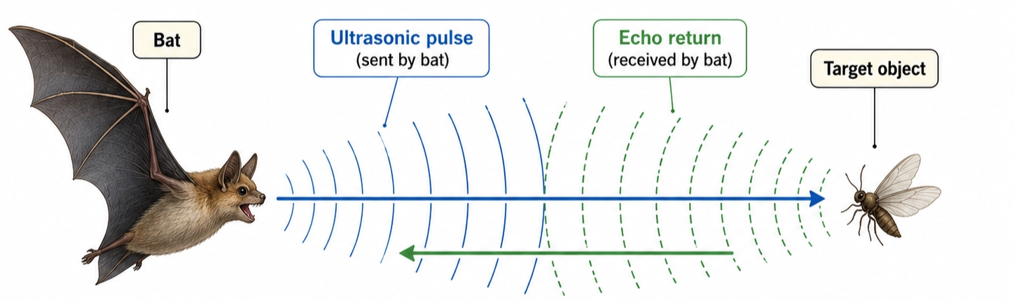
Traditional pulse radars almost do the exact same thing, but with radio waves instead of sound waves: it sends out short bursts of radio waves (at a set carrier frequency, like 10GHz) and measures the time delay before it receives the 'echo'.

A simple pulse radar cycle is:

1. Transmit a short RF pulse

2. Stop transmitting and listen

3. Receive the echo reflected from an object

4. Measure the delay

5. Convert delay into range using the range formula:

   $R=\frac{c \cdot t}{2}$

   where R is the distance to target, c is the speed of light, and t is the measured time delay.

Shortcomings of Traditional Pulsed Radar

Since RF waves travel at the speed of light (they exist on the electromagnetic spectrum), short distances correspond to extremely tiny time delays.

For example, an object 1 meter away creates a round-trip delay of only:

$t=\frac{2R}{c}=\frac{2(1)}{3 \times 10^8}≈6.7 ns$

So to measure nearby objects accurately, a pulse radar needs very fast timing electronics.

Furthermore, in a traditional pulsed radar, the same antenna or RF front end often has to switch between transmit mode and receive mode. During and immediately after the transmit pulse, the receiver may be blanked or recovering from the strong transmit signal.

That creates a minimum detection range. Very close objects can reflect back while the radar is still transmitting or while the receiver is not ready.

So pulse radar is naturally good for longer-range applications, but can be awkward for close-range sensing. In the next section, we will explain how modern mmWave overcomes these problems.

FCMW: How modern mmWave works

mmWave radar, as its name suggests, uses extremely high-frequency radio waves that result in millimeter-scale wavelengths (as per the wavelength formula, $\lambda = \frac{v}{f}$). But traditional radars can do that too, operating at many frequencies from lower microwave bands with centimeter-scale wavelengths to mmWave bands with millimeter-scale wavelengths. So why is modern mmWave radar different?

The key lies in the way distance is measured. Most modern mmWave radar modules transmit FMCW (Frequency Modulated Continuous Wave) signals. Instead of sending out a single short "ping" and directly measuring how long it takes to return, an FMCW radar sends a continuous signal whose frequency changes over time. This changing signal is called a chirp.

A chirp is like a slide whistle moving from a low note to a high note. The radar rapidly sweeps its transmit frequency upward across a known range of frequencies. For example, a radar may start at one frequency, increase smoothly over a few microseconds, then reset and repeat the sweep many times per second.

The basic range measurement works like this:

1. The radar transmits a chirp.
2. The chirp travels outward at the speed of light.
3. The signal hits an object, such as a wall, vehicle, drone, or person, and part of the energy reflects back.
4. By the time that reflection returns, the radar is already transmitting a slightly higher frequency than it was when the signal first left.
5. The radar compares the received echo with the signal it is currently transmitting.
6. The difference between those two frequencies is called the beat frequency.

For example:

Current transmitted frequency: 77.010 GHz

Returning delayed frequency: 77.008 GHz

Difference: 2 MHz

This beat frequency is directly related to distance. A nearby object produces a small delay, so the returned signal is only slightly behind the outgoing chirp. That creates a smaller frequency difference. A farther object produces a larger delay, so the returned signal is farther behind the outgoing chirp. That creates a larger frequency difference.

In other words, FMCW radar turns a very tiny time delay into a frequency difference that is much easier to measure electronically.

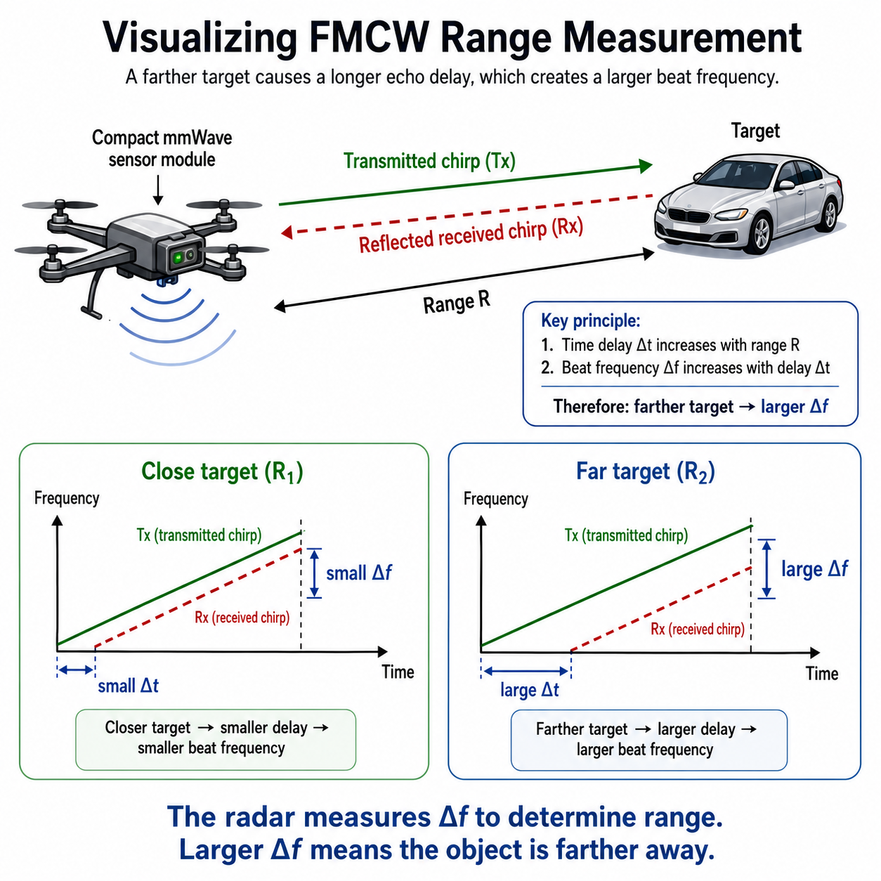
This is one of the major advantages of FMCW radar. Radio waves travel extremely fast, so direct time-of-flight measurements over short distances are difficult. For example, an object only one meter away reflects a signal back in about 6.7 nanoseconds. Measuring that delay directly requires extremely fast timing hardware. FMCW radar avoids this problem by measuring frequency difference instead of directly measuring nanosecond-scale delays.

What affects max range?

There are 3 main things that affect the max range of a mmWave radar:

Chirp Slope

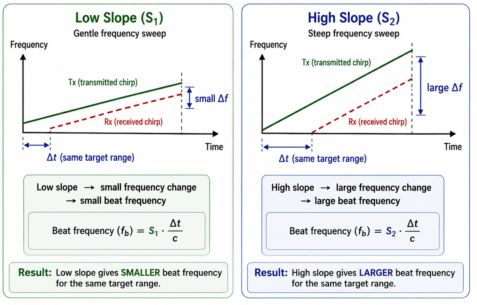
The chirp slope (or frequency slope), measured in MHz or GHz, represents how fast the chirp frequency increases. Visually, it is quite literally the slope of the frequency/time graph. For instance, if your frequency slope is set to 70, that means that your chirp frequency increases 70 MHz every microsecond.

The faster the transmit frequency changes, the larger the beat frequency becomes for a given distance. A steeper slope makes nearby objects easier to distinguish but also increases the beat frequencies that the receiver must measure.

At this point, you may be wondering:

"If the target is at the same distance, shouldn't the radar compute the same answer regardless of the slope?”

And you would be right—the distance estimate is the same. However, this parameter becomes more complex because we also need to consider how easy it is for the radar electronics to measure that distance. This creates an interesting tradeoff between ADC frequency and chirp slope, which will be discussed later in the tradeoffs section.

Time Delay

This one is not a parameter, but rather correlates directly with the physical distance between the object and the radar. Time delay is what creates the beat frequency, allowing you to calculate the range in the first place.

To put it simply, objects farther away take longer to reflect the signal. A longer delay creates a larger beat frequency, resulting in a greater measured distance.

ADC Sampling

The beat frequency must be sampled by the ADC (Analog-to-Digital Converter). This is different from the transmitted frequencies (which are determined by the frequency/chirp slope): the ADC sampling frequency is limited by the hardware's processing speeds and the RX (receiving) antenna.

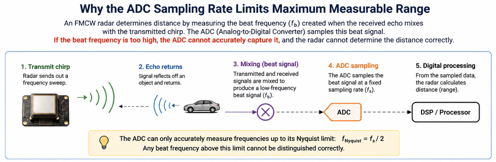
If the beat frequency exceeds what the ADC can accurately capture (its effective Nyquist limit), the radar can no longer distinguish that target correctly. This is one of the reasons maximum measurable range is limited.

How to calculate range

Earlier, we learned that the radar measures the beat frequency: the frequency difference between the transmitted and received chirps.

But how does the radar convert that beat frequency into an actual distance?

The answer comes from two simple relationships.

1. Farther objects create a larger time delay

   Imagine a target 10 meters away. The radar signal doesn't just travel 10 meters. It must travel:

   • 10 meters to the object
   • 10 meters back to the radar

   The total distance traveled is therefore 20 meters.

   Because radio waves travel at the speed of light (ccc), the round-trip delay is

   $$\Delta t=\frac{2R}{c}$$

   where:

   • R = distance to the target
   • c = speed of light

   This means:

   • A nearby object produces a small time delay
   • A distant object produces a larger time delay

2. The chirp converts that delay into a beat frequency

   During this delay, the radar continues sweeping upward in frequency.

   If the chirp is changing frequency at a rate of $S$ Hz/s (the chirp slope), then a delayed signal will return at a lower frequency than the signal currently being transmitted.

   

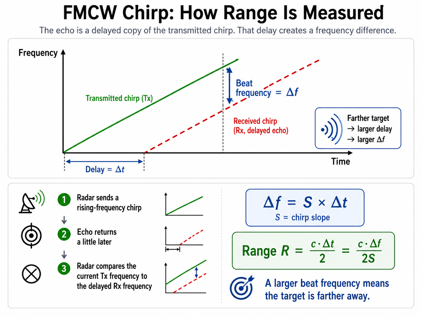
   The frequency difference is simply

   $$f_b=S\Delta t$$

   where:

   • $f_b$ = beat frequency
   • $S$ = chirp slope
   • $\Delta t$ = round-trip time delay

   This tells us that the farther away the object is, the larger the beat frequency becomes.

3. Combine the two equations

   We now know $\Delta t=\frac{2R}{c}$ and $f_b=S\Delta t$.

   Substituting the first equation into the second gives

   $$f_b=S\left(\frac{2R}{c}\right)$$

   Now, solve for range $R$:

   $$R=\frac{cf_b}{2S}$$

   This is the fundamental range equation used by FMCW radar.

The radar already knows the chirp slope because it generated the chirp itself. It then measures the beat frequency using the ADC. Once it knows both values, calculating the distance is straightforward.

But this is just the range equation for the range/distance of a singular detected point. A much more useful number in application would be the max possible range of the radar, which depends on the ADC sampling rate.

If your ADC samples at $F_s$ samples/second, then by the Nyquist theorem (which states that to accurately record and perfectly reconstruct an analog signal, you must sample it at a rate strictly greater than twice the highest frequency component present in that signal), the highest frequency you can uniquely measure is:

$${F_{bmax}}=\frac{F_s}{2}$$

Now substitute that into the first equation:

$$R_{\max}=\frac{c}{2S}\left(\frac{F_s}{2}\right)$$

which simplifies to

$$\boxed{R_{\max}=\frac{cF_s}{4S}}$$

This equation gives you the maximum range of a FMCW radar, given the chirp slope $S$ and ADC sampling frequency $F_s$.

Tradeoffs related to range

Increasing a radar's maximum range may seem straightforward. Looking at the maximum measurable range equation that we just calculated,

$${R_{\max}=\frac{cF_s}{4S}}$$

it appears there are only two options:

• Increase the ADC sampling frequency $F_s$
• Decrease the chirp slope $S$

However, neither parameter can be adjusted indefinitely. Both are constrained by the physical capabilities of the radar hardware, and changing one often affects other aspects of radar performance.

Option 1: Increasing the ADC Sampling Rate $F_s$

A higher ADC sampling rate allows the radar to measure higher beat frequencies before aliasing occurs. Since distant targets produce larger beat frequencies, increasing $F_s$increases the maximum measurable range.

This seems like an obvious improvement, but several hardware limitations prevent arbitrarily high sampling rates.

For BotBlox's mmWave Core module, the maximum effective ADC Sampling rate is ~30 MSPS. This is a hardware limitation and cannot be bypassed.

1. Sampling speed

   Every ADC has a maximum sampling rate determined by its internal electronics. For example, a radar with a 25 MSPS ADC cannot simply be configured to sample at 100 MSPS. Faster ADCs require:

   • more sophisticated analog circuitry
   • lower timing jitter
   • higher power consumption
   • more silicon area
   • higher manufacturing cost

   These practical limitations set an upper bound on $F_s$.

2. Data Throughput

   Every ADC sample becomes digital data that must be stored and processed. This means that doubling the sampling rate doubles the amount of data generated each second.

   For example, increasing the sampling rate from 10MSPS to 40MSPS creates four times as much data that must be transferred, buffered, and processed in real time.

   This places increasing demands on:

   • memory bandwidth
   • DMA transfers
   • DSP performance
   • FPGA or processor resources
   • communication interfaces

   Eventually, the processing hardware becomes the bottleneck rather than the ADC itself.

3. Power Consumption

   Higher-speed ADCs consume more electrical power. Additional power results in:

   • increased heat generation
   • reduced battery life
   • more demanding thermal management

   For compact embedded radar systems, thermal limits often become just as important as electrical limits.

4. Analog Front-End Bandwidth

   The ADC is only one part of the receiver chain. Before reaching the ADC, the beat signal passes through:

   • mixers
   • amplifiers
   • low-pass filters

   These analog components also have finite bandwidth. Even if the ADC could sample extremely high frequencies, the analog circuitry may significantly attenuate those frequencies before they ever reach the converter.

Option 2: Decreasing the Chirp Slope $S$

Another way to increase maximum range is to reduce the chirp slope. A smaller slope causes the transmit frequency to change more slowly, so the same propagation delay produces a smaller beat frequency. This allows distant targets to remain within the measurable frequency range of the ADC.

However, reducing the chirp slope introduces its own limitations.

1. Reduced Range Resolution

   A lower chirp slope typically means less bandwidth over the duration of a chirp.

   Range resolution (to be discussed in the next section) is determined by the total transmitted bandwidth:

   $$\Delta R=\frac{c}{2B}$$

   where $B$ is the chirp bandwidth.

   Lower bandwidth causes nearby objects to become more difficult to distinguish. Two closely spaced targets may merge into a single detection. This is one of the most important tradeoffs in FMCW radar:

   Increasing maximum range generally reduces range resolution.

2. Longer Chirps

   If high bandwidth must be maintained while reducing slope, the only option is to make the chirp longer.

   Since

   $$B=S\times T_{\text{chirp}}$$

   reducing $S$ while keeping $B$ constant requires you to increase the chirp duration, $T_{chirp}$.

   Longer chirps increase:

   • frame duration
   • latency
   • motion sensitivity

   They may also reduce the achievable frame rate.

3. Motion Effects

   Longer chirps allow fast-moving objects to change position more during a single chirp.

   This can introduce:

   • Doppler coupling
   • range migration
   • additional signal-processing complexity

   High-speed automotive radars therefore cannot simply make chirps arbitrarily long.

Other Limits

Even if the radar could measure extremely large beat frequencies and transmit arbitrarily long chirps, maximum detection range would still be limited by physics.

Eventually, the reflected signal becomes too weak to detect.

Detection range depends on:

• transmit power
• antenna gain
• receiver noise figure
• radar cross section (RCS)
• atmospheric attenuation
• detection thresholds (CFAR)

Many of which will be discussed in the Technical Fundamentals section. These factors determine whether the radar can detect a target at all, regardless of the theoretical maximum measurable range.

Summary of Tradeoffs

Change	Benefit	Tradeoff
Increase ADC sampling rate $F_s$	Increases maximum measurable range	Higher power consumption, increased data rate, greater processing requirements, limited by ADC and analog front-end bandwidth
Decrease chirp slope $S$	Increases maximum measurable range	Lower beat frequencies, but reduced range resolution unless chirps are made longer